Consumer electronics based smart technologies for enhanced terahertz healthcare having an integration of split learning with medical imaging

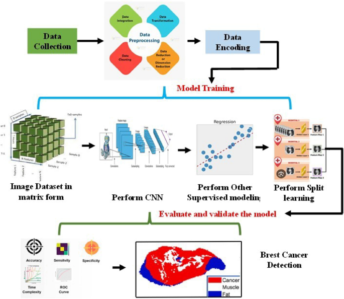
The entirety of the proposed model’s architecture is composed of three distinct components. The initial component entails data collection, which is executed via the utilization of smart consumer electronics-based data collection employing an IoT-based system or a wearable sensor. The subsequent phase entails the provision of guidance and the subsequent evaluation and validation of the outcomes of the model. With regard to instruction, the EM optimized algorithm has been utilized, while the Bayesian-based split learning model has been employed for the anticipation of breast cancer.
Preprocessing for Data Analysis and Materials/Methods in the context of using terahertz (THz) imaging for breast can- cer identification involves several key steps: such as data collection and acquisition, preprocessing of data, feature extraction, and splitting.
Data acquisition
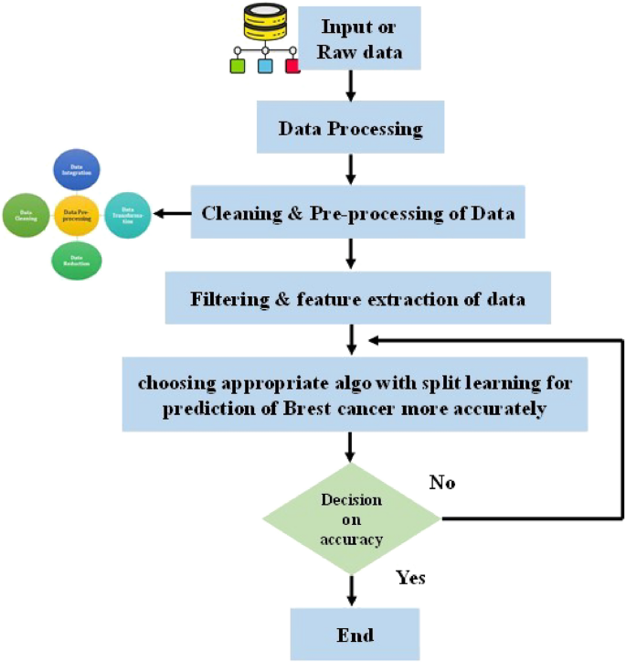
In Data Acquisition, the gather THz imaging data from recently removed mouse tumors, ensuring that the data is accurately recorded and properly labeled for breast cancer identification. This module is employed for the purpose of eliminating any form of noise or artifacts that may be present in the THz data, thereby guaranteeing that the dataset is devoid of any anomalies that might have a detrimental impact on the performance of the model. At present, there exists a necessity to identify a suitable feature, a requirement that is met by the feature extraction method. Consequently, it becomes imperative to ascertain the pertinent features or characteristics from the THz images, which can subsequently be utilized as input variables for the models. This may involve techniques such as edge detection or texture analysis. In the very next level, it has been dividing the dataset into training and testing sets to assess model performance. Given that the approach aims to reduce the demand for extensive training data, this splitting should be designed to optimize data uses (see Figs. 1 and 2).

Architecture of newly proposed healthcare prediction system using split learning method.

Step by step process from collection of data to choosing appropriate model with split learning for predict the health- care condition, the whole method.
The mathematical equation for data acquisition can be represented using the concept of sampling. Data acquisition typically involves sampling a continuous signal at discrete time intervals. The equation for data acquisition is often expressed as:
$$x[n] \, = x(t_n ) \, = f(nT_s )$$
(1)
where x[n] is the sampled data at the discrete time index n, x(tn) represent the continuous signal x(t), sampled at a specific time tn, F(nTS) is the function that samples the continuous signal x(t) at discrete time interval. “n” is the index of the discrete samples; TS is the sample interval. This equation describes how continuous data is converted into a discrete form through sampling. The choice of the sampling interval TS is critical and is determined by the Nyquist-Shannon sampling theorem, which states that TS should be less than or equal to half the reciprocal of the highest frequency component present in the signal to avoid aliasing.
Preprocessing of the raw data
In this section, it has been discussing the pre-processing method, which contain from sampled data to normalized, scaled etc. Once it has been getting the data, the preprocessing encompasses various steps such as normalization, imputation, and scaling. The whole process is shown in Fig. 2, which started from raw data to the choosing an appropriate model. The mathematical equation for a common preprocessing step, min–max normalization, can be represented as:
$$X_normalized = \frac\textx – \textmin(x)maz(x) – min(x)$$
(2)
where x is the actual/ original data point, Xnormalized is the normalized data point, min(x) and max(x) are the minimum and maximum value in the data set. After getting the normalized value filter is used to remove the unwanted data from the signal. Here we have to choose which type of filter is used, it may be a low pass or high pass filter as per the requirement. Here a simple mathematical representation of a low pass filter is given
$$Y(t) = \int x \cdot t^t \sum h(t – t^t ) dt^t$$
(3)
where, y(t) is the filter signal, x(t) is the original signal, h(t) is the impulse response of the filter signal.
Feature extraction
Once the scaled data is obtained, it becomes necessary to identify the suitable feature from this data. Due to the presence of numerous parameters in the data, the PCA method is employed to identify the relevant data that can aid in predicting the healthcare status. In the subsequent discussion, we will elaborate on the step-by-step process of PCA for feature extraction and which is shown in Fig. 1. This figure tells detail about starting from choosing of raw data, filter process, feature extraction (PCA method), and finally considering appropriate training, testing and validation model.
After the completion of the filtering stage, it is necessary to carry out the process of feature extraction. The purpose of feature extraction is to convert the data into a collection of pertinent features. Principal Component Analysis (PCA) is a widely used method for reducing the dimensionality of the data and extracting features. The mathematical formula for PCA involves the identification of the principal components through eigen decomposition.
where X is the original data, which represented as in the matrix form. W is the is the principal component (matrix of eigenvectors). Z is the is the transformed data having reduced dimensionality and represented in the form of matrix. PCA seeks to find W such that the transformed data Z retain the X-dimensionality. For the next step it has consider X as input data.
Implement with appropriate algorithm with split learning
In this section, we have amalgamated the split learning technique with the machine learning model to facilitate the early identification of breast cancer through the utilization of terahertz medical imaging. Within the machine learning model, we have employed the Bayesian approach to forecast the occurrence of breast cancer. The incorporation of split learning methodology ensures the privacy of sensitive and confidential patient information. Subsequently, an elaborate explanation of the newly proposed mathematical model and the intricate details of the split learning-based hybrid algorithm will be discussed below.
A newly proposed model, integrating with split learning for early detection breast cancer using terahertz medical imaging.
Training the machine learning model is of utmost importance to predict breast cancer accurately. The model’s accuracy is heavily dependent on the quality of the training data. In this study, FFPE samples22 were used as a reference point for the training purposes. However, the dehydration process can negatively impact the quality of the training data due to differences in shape between freshly excised samples and their FFPE counterparts. To overcome this challenge, we propose an innovative approach, such as the EM algorithm, which aims to select training data based on reliability.
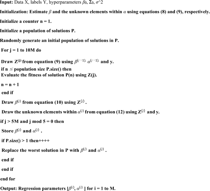
Once we train the machine learning model, now we can used the appropriate algorithm to predict the breast cancer. For the model terahertz (THz) imaging of the given mouse data is act as input. And we can used this data to the proposed supervised multinomial Bayesian with split learning for the identification of breast cancer. One more advantages of this model is, it requires only a small set of model parameters compare to other proposed models22. Detail of the mathematical model of the proposed algorithm can see module.Algorithm: Hybrid Training Procedure using split learning.

Algorithm: Hybrid Training Procedure using split learning.
Development of split learning model
Mathematically formulating the split learning algorithm for predicting healthcare diseases necessitates the articulation of the fundamental elements and procedures of the algorithm in mathematical symbols. Here it has lies a comprehensive mathematical representation of the split learning procedure:
As lastly, we have obtained the featured input data X, which is represented in a matrix of size n × m, where n is the number of samples (patients/ mouse) and m is the number of features (attributes/ parameters). Let Y represent the predicted value as output for the given input data X. So that the input X, in the form of function Fc defined as
$$F_c = (X;\theta_c )$$
(5)
where Fc represents the input model function with parameters θc. This model extracts features from the input data.
Similarly the Fs the output function parameters θs can defined as
$$F_s = (F_c (X;\theta c);\theta_s )$$
(6)
This model makes the final disease predictions based on the features extracted by the input model. The split learning process involves iterative communication rounds between the input and output models until convergence: In each iteration, the input model updates its features using the following equation:
$$X^j = Fc(X;\theta_c )$$
(7)
The output model takes these features and makes predictions:
$$Y^t = Fs(X^t ;\theta s )$$
(8)
The input model updates its parameters using the predictions and a loss function
$$\theta c \leftarrow \theta c – \alpha \nabla \theta cL(Y^t ,Y)$$
(9)
Similarly the output model also updates its parameters using the same loss function:
$$\theta s \leftarrow \theta s – \alpha \nabla \theta sL(Y^t ,Y)$$
(10)
This process continues until convergence, where α is the learning rate. After achieving convergence, the ultimate pa- rameters of the global model are acquired through the process of the parameters of the model at the input and output function. Appropriate evaluation metrics can be utilized to evaluate the efficiency of the model, encompassing accuracy, precision, recall, and F1-score, amongst others. The aforementioned mathematical modeling offers a comprehensive framework for comprehending the split learning algorithm employed in healthcare disease prediction.
Testing process in the proposed model
In order to determine whether there is a significant difference between the average values of cancerous and non-cancerous pixels within each test sample using our proposed model. The first step was to conduct a univariate t-test. This analysis used the first component of the low-dimensional vector per pixel, which was obtained from the output of the proposed algorithm.
The null hypothesis of this t-test assumes that there are equal means between the outputs of cancerous and non-cancerous pixels. Table 1 presents the results of the t-test, which showed that the p-values for all test samples were almost zero. This indicates that the null hypothesis can be rejected, confirming that there are significant differences in the mean values of the outputs of cancerous and non-cancerous pixels, as revealed by the t-test results.
link


