Multi-objective trajectory optimization method for industrial robots based on improved TD3 algorithm

A Markov Decision Process (MDP) is a sequential decision-making mathematical model24 used to simulate an agent’s stochastic policy and rewards in a Markovian environment. As the fundamental mathematical framework of deep reinforcement learning, an MDP must be established when solving robotic arm trajectory planning problems using deep reinforcement learning methods. MDP comprises five key elements \(\{S, A, P_{sa}, \gamma , R\}\), where \(P_{sa}\) represents the state transition function and \(\gamma\) is the discount factor. In the Markov Decision Process, the agent selects actions through interactions with the environment, with each decision influencing the system’s state.
The decision-making process for industrial robot trajectory planning can be abstracted as a Markov Decision Process, where continuous interactions occur between the industrial robot and its environment. By employing reinforcement learning algorithms to train industrial robots in decision-making related to joint angular velocities, the robot can autonomously select a trajectory with significant reward value, achieving a collision-free, highly smooth, and time-optimal trajectory for industrial robots.
A quintuple \(\{S, A, P_{sa}, \gamma , R\}\) is used to describe the decision-making process of industrial robot trajectory planning. In one episode, the industrial robot receives state space information S from the environment, including distance information, posture information, angular information of six joints, and collision status information. The industrial robot then selects actions A The probability of the industrial robot transitioning to the next state based on action A in state S is referred to as the state transition probability \(P_{sa}\). (angle changes for the six joints) based on the received information, and the corresponding actor network is updated through algorithm training. To balance current and future rewards, a discount factor \(\gamma\) is introduced in the trajectory planning decision-making process to prevent the algorithm from entering infinite loops and to ensure convergence. When \(\gamma\) approaches 1, the importance of future rewards increases, whereas when \(\gamma\) approaches 0, the importance of current rewards dominates. The industrial robot receives a numerical reward R, which serves as the immediate return when the agent transitions from state S to state \(S’\) after taking action A. Rewards are typically used to measure the quality of a state-action pair.
In industrial robot trajectory planning within confined environments, the Markov property refers to the robot selecting the optimal action at each time step based on the current state, which includes the surrounding environmental state and its own position and posture information. After executing the action, the robot perceives changes in the environment and updates its own state to receive a feedback reward (return value). Based on the reward, the robot adjusts its next action and continues this process until an optimal policy is formed. The Markov property emphasizes that the choice of the current state depends solely on the current environmental state and not on past historical information.
Observation and action space setup
When training a DRL algorithm for an industrial robot, it is essential to define its state space and action space. Therefore, a reasonable state space must be designed for the robot and its environment to generate input data for the neural network. In the trajectory planning task of this paper, the state information mainly includes two aspects: environmental information and self-information. Environmental information includes collision detection between the robot and obstacles, the distance between the robot and the target point, and the deviation between the robot’s posture and the target posture. Self-information includes the angles of the six joints, whether the robot has reached the target position, and whether the robot has achieved the target posture. The posture of the robot’s end-effector is represented using quaternions, which effectively avoids the issue of gimbal lock25. The deviation between the posture of the robotic arm’s end-effector and the target posture can be quantitatively described using the Axis-Angle Representation. This method uses a rotation axis and rotation angle to represent the difference between the two, providing an accurate geometric representation that facilitates the adjustment and optimization of the end-effector’s posture. In this paper, the rotation angle is used to quantitatively analyze the deviation between the robot’s end-effector posture and the target posture. Therefore, the state \(s_t\) is defined as:
$$\begin{aligned} s_t = [A,P,D,T] \end{aligned}$$
(1)
In the above equation, A represents the joint angles of the robotic arm in its current state. For the 6-DOF robotic arm selected in this paper, \(A = [\theta _1, \theta _2, \dots , \theta _6]\). \(P = [x_t, y_t, z_t, q_x, q_y, q_z, q_w]\) represents the three-dimensional positional information and four-dimensional orientation information of the robotic arm’s end-effector in the world coordinate system. \(D=[\Delta x, \Delta y, \Delta z, \Delta \theta ]\) represents the positional and orientation deviations between the robotic arm’s end-effector and the target object. \(T=[bool_{collision},bool_{position},bool_{pose}]\) consists of three Boolean values indicating whether all joints of the robotic arm are in collision with obstacles, whether the arm has reached the target position within the allowable error, and whether the arm has reached the target pose within the allowable error. A value of 1 denotes “yes”, and 0 denotes “no”. A collision state is determined when the distance between the robot and the obstacle is less than 0.05 m. The robot is considered to have reached the target position when the distance between the end-effector and the target position is less than 0.01 m. The robot is considered to have reached the target pose when the axis-angle deviation between the end-effector’s orientation and the target orientation is less than 0.01 radians.
To achieve inverse-kinematics-free trajectory planning for the robotic arm, the action defined in this paper directly controls the joint angles of the robotic arm, where the action \(a_t\) is defined as:
$$\begin{aligned} a_t = [\Delta a_1, \Delta a_2, \dots , \Delta a_6] \end{aligned}$$
(2)
Here, \(\Delta a_n\) corresponds to the rotational increment of the n-th joint angle of the robotic arm. Based on the above equation, the agent determines the increments of the six joint angles of the robotic arm according to the current state \(s_t\) and the policy, causing changes in the position and posture of the end-effector. Since all joint angles are known, the unique position and posture of the end-effector can be determined using the forward kinematics of the robotic arm. This eliminates the need for complex inverse kinematics calculations, effectively avoiding the common issue of singularities and ensuring that every point in the trajectory generated by the agent is reachable by the robotic arm. When generating action, certain kinematic constraints must be satisfied, meaning that at any given moment, the robot’s joint angles, joint angular velocities, and angular accelerations must not exceed the robot’s maximum allowable limits. The specific constraints are shown in Eq. (3).
$$\begin{aligned} {\left\{ \begin{array}{ll} |\theta _i(t)| \le \theta _{max} & \forall t \in [t_i, t_{i+1}] \\ |\theta _i'(t)| \le \theta _{max}’ & \forall t \in [t_i, t_{i+1}] \\ |\theta _i”(t)| \le \theta _{max}” & \forall t \in [t_i, t_{i+1}] \end{array}\right. } \end{aligned}$$
(3)
Reward function design
The essence of Deep Reinforcement Learning (DRL) lies in processing input state information through neural networks under the guidance of a reward function and establishing the relationship between state, value estimation, and decision-making. In DRL applications, the design of the reward function is crucial. By converting task objectives into mathematical forms, effective communication between the task and the algorithm is achieved, determining whether the agent can learn the required skills and directly influencing the algorithm’s convergence speed and robustness.

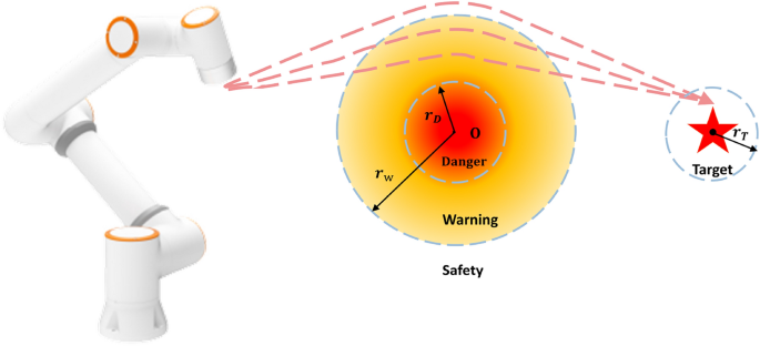
Danger zone division in the industrial robot’s workspace.
In past studies, the reward for robot trajectory planning typically relied only on the deviations in position and posture, with fixed weight coefficients for position and posture. This approach fails to adequately account for state changes between consecutive time steps and cannot dynamically adjust weights based on the current workspace, thereby limiting the convergence speed. As shown in Fig. 1, the workspace around the obstacle is divided into three parts: a safe zone, a warning zone, and a danger zone. Here, \(r_D\) and \(r_W\) represent the radii of the danger zone and warning zone, respectively, while \(r_T\) represents the radius of the target zone. The positional deviation between the industrial robot’s end-effector and the target point can be represented by the Euclidean distance \(d_t\). The reward function \(R_t\) can be defined as:
$$\begin{aligned} d_t=\sqrt{(x_t – x_g)^2 + (y_t – y_g)^2 + (z_t – z_g)^2} \end{aligned}$$
(4)
Here, \((x_t,y_t,z_t )\) and \((x_g,y_g,z_g )\) represent the current position of the robot’s end-effector and the target position respectively.
The orientation deviation is calculated using quaternions, starting with the computation of the conjugate quaternion \(q^*_t\) of the current end-effector orientation:
$$\begin{aligned} q^*_t=[-q_{xt},-q_{yt},-q_{zt},q_{wt}] \end{aligned}$$
(5)
Then calculate the relative quaternion \(q_{relative}\) between the current orientation and the target orientation:
$$\begin{aligned} q_{relative}= & q^*_t \cdot q_g = [-q_{xt},-q_{yt},-q_{zt},q_{wt}] \cdot [q_{xg},q_{yg},q_{zg},q_{wg}] \nonumber \\= & [q_{x\_relative},q_{y\_relative},q_{z\_relative},q_{w\_relative}] \end{aligned}$$
(6)
Finally, the rotation angle \(\theta\) between the current orientation and the target orientation can be determined based on the relative quaternion:
$$\begin{aligned} \theta = 2 \cdot \arccos (q_{w\_relative}) \end{aligned}$$
(7)
\([q_{xt},q_{yt},q_{zt},q_{wt}]\) and \([q_{xg},q_{yg},q_{zg},q_{wg}]\) represent the current orientation and the target orientation of the robot’s end-effector, respectively.
The positional deviation between each joint of the industrial robot and the obstacles can be represented by the Euclidean distance \(d_{oi}\):
$$\begin{aligned} d_{oi}=\sqrt{(x_{oi}-x_o)^2+(y_{oi}-y_o)^2+(z_{oi}-z_o)^2} \end{aligned}$$
(8)
When detecting whether the robot has collided with an obstacle, the shortest distance between any joint and the obstacle is taken as the robot’s collision detection distance, \(d_o = \min _i d_{oi}\).
This paper employs a reward shaping method26 to avoid the issue of sparse rewards. Based on the optimization principles proposed earlier and real-world reward requirements, a composite reward function is designed by comprehensively considering factors such as distance, orientation, time steps, path length, joint angles, motion speed, and path smoothness, as shown below:
$$\begin{aligned} R = R_a + R_s + R_t + R_l + R_o + R_{suc} \end{aligned}$$
(9)
The composite reward function consists of six main components: \(R_a\), \(R_s\) and \(R_t\), which guide the robotic arm to generate a collision-free, smooth, and time-optimal trajectory; \(R_l\), which controls the path length; \(R_o\), which penalizes proximity to obstacles; and \(R_suc\), which rewards reaching the target object with the specified position and orientation. \(R_a\) (Precision Reward):Dense shaping rewards are provided based on reducing position and orientation deviations, directly promoting execution time optimization. The dynamic adjustment factor \(\alpha _{dis}\) ensures a smooth transition from prioritizing position to prioritizing orientation as the end-effector approaches the target, thereby improving final precision. \(R_s\) (Smoothness Reward) and \(R_l\) (Path Length Reward): These components are crucial for satisfying kinematic constraints. By penalizing large joint angles and high angular velocities (\(R_s\)) and encouraging shorter paths (\(R_l\)), the reward function inherently promotes smoother motion, which is less likely to violate the robot’s speed and acceleration limits. \(R_t\) (Execution Time Optimization Reward):Since the simulation used in this paper is a fixed-step simulation, the reward guides the industrial robot to move from the starting pose to the target pose with the smallest time steps, thereby achieving execution time optimization. \(R_o\) (Obstacle Penalty) and \(R_{suc}\) (Success Reward): These components are fundamental to ensuring collision-free motion. Severe penalties are imposed for behaviors that enter the danger zones around obstacles, strongly discouraging unsafe trajectories. A large positive reward provides a clear incentive for successfully reaching the target without collision.
When designing the reward function \(R_a\) to guide the robot to reach the target with the specified position and orientation, we choose the negative of the positional deviation between the robotic arm’s end-effector and the target position, as well as the orientation deviation between the end-effector and the target, as the potential function.
$$\begin{aligned} \phi (s) = -(\alpha _{dis} \cdot |P – G| + (1 – \alpha _{dis}) \cdot \theta ) \end{aligned}$$
(10)
In the equation, \(\alpha _{dis}\) is a dynamic adjustment factor for the weight of the positional deviation. This paper introduces \(\alpha _{dis}\) to help guide industrial robots in balancing exploration and exploitation during trajectory planning, thereby improving policy convergence speed and precision. When the distance to the target position is large, the position deviation dominates the \(R_a\) reward function; as the distance to the target decreases, the weight of position deviation gradually decreases, and the orientation deviation gradually takes precedence. The setting of \(\alpha _{dis}\) is as follows:
$$\begin{aligned} \alpha _{dis} = {\left\{ \begin{array}{ll} \alpha _{initial} & \text {if } d_t \ge d_{threshold} \\ \alpha _{initial} \cdot ((1-\alpha _{initial}) + \alpha _{initial} \cdot \frac{d_t}{d_{threshold} }) & \text {otherwise} \end{array}\right. } \end{aligned}$$
(11)
Under the influence of the potential function27, the target position and orientation become an attractor state. When the robotic arm approaches the target position and orientation, it receives a positive reward; when it moves away, it receives a negative reward. This reduces redundant actions during environmental exploration and accelerates the agent’s learning. Therefore, we define \(R_a\) as follows:
$$\begin{aligned} R_a&= \omega _a * [\alpha _{dis} * (|P_{t-1} – G| – |P_t – G|) + (1 – \alpha _{dis}) * (\theta _{t-1} – \theta _t)] \nonumber \\&=\omega _a * [\alpha _{dis} * (d_{t-1} – d_t) + (1 – \alpha _{dis}) * (\text {angle}_{t-1} – \text {angle}_t)] \end{aligned}$$
(12)
In the equation, \(P_t\) and \(\theta _t\) represent the position and orientation deviations of the industrial robot’s end-effector at the current time step, while \(P_{t-1}\) and \(\theta _{t-1}\) are the position and orientation deviations at the previous time step. \(\omega _a\) is the weight coefficient of the precision reward designed to achieve the optimization objective of accuracy.
The reward functions for other components are as follows:
The reward function \(R_s\) for path smoothness is defined as:
$$\begin{aligned} R_s = -\omega _s \sum _{k=1}^2 (\lambda _\theta \theta _k^2 + \lambda _v {\dot{\theta }}_k^2) \end{aligned}$$
(13)
The reward function \(R_t\) for time optimization is:
$$\begin{aligned} R_t = \omega _t(\frac{max\_steps\_one\_episode – step\_counter_t}{max\_steps\_one\_episode})^2 \end{aligned}$$
(14)
The reward function \(R_l\) for path length control is:
$$\begin{aligned} R_l = \omega _l(\frac{\rho – path\_length_t}{\rho })^2 \end{aligned}$$
(15)
The reward function \(R_o\) for obstacle avoidance is:
$$\begin{aligned} R_o = {\left\{ \begin{array}{ll} -100 & \text {if } d_o \le r_D \\ -\mu + \max (r_W – d_o, 0) & \text {otherwise} \end{array}\right. } \end{aligned}$$
(16)
The reward function \(R_{suc}\) for successful target reaching is:
$$\begin{aligned} R_{suc} = {\left\{ \begin{array}{ll} 2000 & \text {if } d_t \le r_T \text { and } \theta \le \theta _T \\ 0 & \text {otherwise} \end{array}\right. } \end{aligned}$$
(17)
\(\omega _s\) and \(\omega _t\) represent the weight coefficients set to achieve the optimization objectives of smoothness and time optimality respectively, and \(\omega _l\) represents the weight coefficient for optimizing path length. \(\lambda _\theta\) and \(\lambda _v\) are the weight coefficients for joint angles and joint angular velocities, used to smooth actions and improve path quality. \(\theta _k\) and \({\dot{\theta }}_k\) represent the joint angle and angular velocity of the k-th joint respectively. \(max\_steps\_one\_episode\) refers to the maximum number of time steps per episode, and \(step\_counter_t\) represents the current time step. \(\rho\) is the path length parameter set based on experiments, and \(path\_length_t\) represents the robot’s path length at the current time step. The parameters related to the composite reward function are shown in Table 1. In this study, the design of the reward function considers multiple factors to balance objectives such as time optimization, path quality optimization, and collision avoidance.
Specifically, the selection of weights is based on the following considerations: \(\omega _a\) (Weight for target position and orientation deviation: 600): We assign a higher weight to Ra primarily to ensure the robot reaches the target position as quickly as possible and reduces deviation from the target trajectory. Since the deviation in target position and orientation is critical for the success rate of task completion, the weight of \(\omega _a\) is relatively high to prioritize this objective. \(\omega _s\) (Weight for path smoothness: 0.14): The weight for \(\omega _s\) is relatively small because kinematic constraints have already been applied to the industrial robot during the action generation phase. Additionally, while smoothness is important, it has a lower priority compared to collision avoidance and execution time optimization for reaching the target. The weight value has been experimentally validated to ensure that smoothness does not compromise the task’s execution efficiency. \(\omega _t\) (Weight for time optimization: 2): The weight for \(\omega _t\) is relatively high because trajectory execution time is critical for improving the efficiency of industrial robots. This value was chosen based on strict requirements for task completion time and has shown good convergence results in experiments. \(\omega _l\) (Weight for path length: 0.5): Path length plays an important role in path planning, but compared to other factors, an appropriate weight value ensures that the robot achieves a reasonable path length without introducing excessive computational burden. The lower weight reflects that path optimization has a limited impact on the overall task.
link


