Calibration of the omnidirectional vision system for robotics sorting system

Table of Contents

System model

The system model was previously described in¹¹ and just a brief overview is presented in this section. World coordinates of the laser plane (X, Y, Z) can be obtained as follows:

$$\begin{aligned} \begin{bmatrix} u\\ v\\ f\left( p \right) \end{bmatrix}\times \begin{bmatrix} r_{1}^{c}&r_{2}^{c}&r_{3}^{c} \end{bmatrix}\begin{bmatrix} r_{1}^{l}&r_{2}^{l}&r_{3}^{l}&t^{l } \end{bmatrix}\begin{bmatrix} X\\ Y\\ Z\\ 1 \end{bmatrix}=0 \end{aligned}$$

(1)

where u, v represent pixel coordinates;$r_{1}^{c}$, $r_{2}^{c}$, $r_{3}^{c}$, $r_{1}^{l}$, $r_{2}^{l}$, $r_{3}^{l}$, $r^{l}$ represent column vectors of the rotation matrix of the camera and transformation matrix of the laser plane respectively. The polynomial f(p) has the following form:

$$\begin{aligned} f\left( p \right)&=a_{0} +a_{2} p^{2} +\cdots +a_{N} p^{N} \end{aligned}$$

(2)

$$\begin{aligned} p&=\sqrt{\left( u-u_{c} \right) ^{2}+\left( v-v_{c} \right) ^{2}} \end{aligned}$$

(3)

where $a_{i}$ are coefficients; N the degree; point $u_{c}$, $v_{c}$ is the center of the image.

The laser emitter has a rigid configuration, consequently distance to the camera is constant: along the Z-axis. Taking into account the aforementioned criteria, for the proposed vision system Eq. (1) can be simplified as:

$$\begin{aligned} \begin{bmatrix} u\\ v\\ f\left( p \right) \end{bmatrix}\times \begin{bmatrix} r_{1}^{c}&r_{2}^{c}&r_{3}^{c} \end{bmatrix}\begin{bmatrix} r_{1}^{l}&r_{2}^{l}&t^{l } \end{bmatrix}\begin{bmatrix} X\\ Y\\ 1 \end{bmatrix}=0 \end{aligned}$$

(4)

Problem

In²³ was presented a novel calibration technique for obtaining extrinsic parameters between the camera and laser plane. This calibration method was based on the use of a three-sides target and has proven its accuracy and reliability in comparison with other calibration methods. In this section, we propose the optimized calibration target and evaluate its robustness and performance compared to previous calibration methods. As can be seen from Fig. 7b, the optimized calibration target consists of two sides, the calibration target from work²³ consists of three sides (see Fig. 7a). We also placed a chessboard between the sides of the target in order to not only calibrate the computer vision system, but also based on a single input image determine the position of the robot in relation to the camera coordinate system.

Calibration procedure

The goal of the extrinsic calibration is to find parameters of the rotation matrix of the camera and transformation matrix of the laser plane respectively. In general form this optimization problem can be formulated as follows:

$$\begin{aligned} \left\{ \begin{matrix} min_{R^{c},R^{l},T^{l} }\left| \right| f (R^{c},\left[ R^{l},T^{l} \right] )\left| \right| ^{2} \\ subject \ to\ f (R^{c},\left[ R^{l},T^{l} \right] )=\begin{bmatrix} u \\ v\\ f\left( p \right) \end{bmatrix}\times R^{c}\left[ R^{l}\mid T^{l} \right] \begin{bmatrix} X \\ Y \\ 1 \end{bmatrix} \\ R^{c}=\left[ r_{1}^{c} \ r_{2}^{c} \ r_{3}^{c} \right] \\ \left[ R^{l}\mid T^{l} \right] =\left[ r_{1}^{l} \ r_{2}^{l} \ t^{l} \right] \end{matrix}\right. \end{aligned}$$

(5)

where $R^{c}$ represents the rotation matrix of the camera and $\left[ R^{l} \mid T^{l} \right]$ represent transformation matrix of the laser plane, consisting of rotation $R^{l}$ and translation $T^{l}$ parts respectively.

An improved calibration target was developed (see Fig. 8) for solving the optimization problem described in Eq. (5). The main advantage of this target is its versatility, as it can be applied to various configurations of a vision system, as well as its flexibility, as it can be simply placed in front of the mobile robot. The proposed target allows an extrinsic calibration to be performed by only capturing a single snapshot, this procedure is explained below.

Extrinsic calibration of the vision system

This section explains the process of obtaining parameters forming the camera rotation matrix $R^{c}$ as described in Eq. (5). In order to carry out the calibration process to obtain camera extrinsic parameters, first of all, pixel coordinates belonging to the border (between white and black regions) of the target are projected by Eq. (4) to the world coordinate system (see Fig. 9a). After that for every parameter, namely for the pitch, roll, and yaw, the optimization is described as a series of Eqs. (6), 7), (8). The pitch is calculated when projected to the world coordinates vectors $\overline{AB}$ and $\overline{DC}$ of the target collinear to each other. This optimization problem can be formulated as follows:

$$\begin{aligned} \left\{ \begin{matrix} min_{pitch}\left\| f(pitch) \right\| ^{2} \\ subject\ to\ f(pitch)=\frac{\overline{AB}_{Y} }{\overline{AB}_{Z}} -\frac{\overline{DC}_{Y} }{\overline{DC}_{Z}} \end{matrix}\right. \end{aligned}$$

(6)

The yaw is calculated when projected to the world coordinates vectors $\overline{AB}$ and $\overline{DC}$ of the target are not rotated around X-axis. This optimization problem can be formulated as follows:

$$\begin{aligned} \left\{ \begin{matrix} min_{yaw}\left\| f(yaw) \right\| ^{2} \\ subject\ to\ f(yaw)=\frac{\overline{AB}_{Y} }{\overline{AB}_{Z}} \cdot \frac{\overline{DC}_{Y} }{\overline{DC}_{Z}} \end{matrix}\right. \end{aligned}$$

(7)

Once the pitch and yaw are known it is possible to calculate the roll. Sides of the calibration target are the same length as well as the extracted border between black and white regions also is the same length. The roll can be found by minimization the difference between length of vectors $\overline{AB}$ and $\overline{DC}$ whereas pitch and yaw obtained during previous steps are constant. This minimization problem can be written as follows:

$$\begin{aligned} \left\{ \begin{matrix} min_{roll}\left\| f(roll) \right\| ^{2} \\ subject\ to\ f(roll)= \left| \overline{AB} \right| -\left| \overline{DC} \right| \end{matrix}\right. \end{aligned}$$

(8)

At this point, pixel coordinates belonging to the border of the target can be projected by Eq. (4) to the world ones with the pitch, roll, and yaw, determined during the calibration procedure (see Fig. 9b). Once the camera is calibrated, we can move to the calibration of the laser plane.

Extrinsic calibration of the laser plane

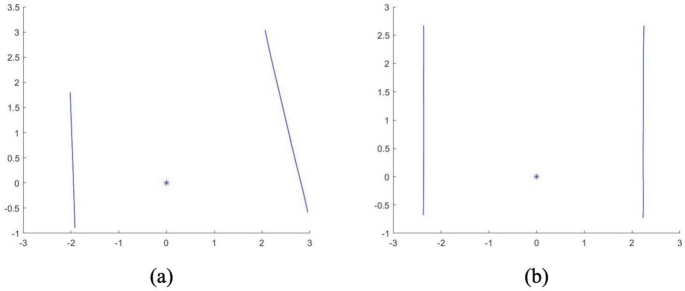
This section outlines the process of obtaining parameters forming the transformation matrix $\left[ R^{l} \mid T^{l}\right]$ of the laser plane, which are part of the Eq. (5), whereas parameters of $R^{c}$ are known and constant. First of all, extracted pixel coordinates of the laser beam are projected by Eq. (4) to the world ones (see Fig. 10a). After that for every parameter related with the transformation matrix of the laser plane, the minimization problem is formulated by a series of Eqs. (9), (10), (11).

The pitch is calculated when projected to the world coordinates vectors $\overline{EF}$ and $\overline{HG}$ of the target collinear to each other. This optimization problem can be formulated as follows:

$$\begin{aligned} \left\{ \begin{matrix} min_{pitch}\left\| f(pitch) \right\| ^{2} \\ subject\ to\ f(pitch)=\frac{\overline{EF}_{Y} }{\overline{HG}_{Z}} -\frac{\overline{EF}_{Y} }{\overline{HG}_{Z}} \end{matrix}\right. \end{aligned}$$

(9)

Another parameter related with the $R^{l}$ is the roll. Sides of the calibration target are the same length as well as the extracted laser strip is also the same length. The roll can be found by minimization the difference between length of vectors ($\overline{EF}$ and $\overline{HG}$ whereas pitch and yaw obtained during previous steps are constant. This minimization problem can be written as follows:

$$\begin{aligned} \left\{ \begin{matrix} min_{roll}\left\| f(roll) \right\| ^{2} \\ subject\ to\ f(roll)= \left| \overline{EF} \right| -\left| \overline{HG} \right| \end{matrix}\right. \end{aligned}$$

(10)

Finally, the last unknown parameter included to the transformation matrix of the laser plane representing the distance to the laser plane can be calculated. The real distance $D_{1}$ between the left and right sides of the target is known. The distance $D_{2}$ between sides of the target can be found experimentally from the world coordinates of the laser. Thus, the depending variable representing the distance to the laser plane can be calculated as the difference between $D_{1}$ and $D_{2}$. This minimization problem can be written as follows:

$$\begin{aligned} \left\{ \begin{matrix} min_{dist}\left\| f(dist) \right\| ^{2} \\ subject\ to\ f(dist)=D_{1}- D_{2} \\ D_{2}=(\frac{Y_{H}+Y_{G}}{2}-\frac{Y_{E}+Y_{F}}{2} ) \end{matrix}\right. \end{aligned}$$

(11)

Afterwards, pixel coordinates of the laser beam can be projected by Eq. (4) to the world ones with the pitch, roll, and distance to the laser plane, determined during the extrinsic calibration (see Fig. 10b).

link